These are solutions to the most recent problems posted for Stanford’s CS 229 course, as of June 2016. I’m not sure if this course re-uses old problems, but please don’t copy the answers if so. This document is also available as a pdf.
1 Problem set 1
1.1 Logistic regression
1.1.1 Part (a)
The problem is to compute the Hessian matrix \(H\) for the function
\[J({\theta}) = -\frac{1}{m}\sum_{i=1}^m\log(g(y{^{(i)}}x{^{(i)}})),\]
where \(g(z)\) is the logistic function, and to show that \(H\) is positive semi-definite; specifically, that \(z^THz\ge 0\) for any vector \(z.\)
We’ll use the fact that \(g'(z) = g(z)(1-g(z)).\) We’ll also note that since all relevant operations are linear, it will suffice to ignore the summation over \(i\) in the definition of \(J.\) I’ll use the notation \(\partial_j\) for \(\frac{\partial}{\partial{\theta}_j},\) and introduce \(t\) for \(y{\theta}^Tx.\) Then
\[-\partial_j(mJ) = \frac{g(t)(1-g(t))}{g(t)}x_jy = x_jy(1-g(t)).\]
Next
\[-\partial_k\partial_j(mJ) = x_jy\big(-g(t)(1-g(t))\big)x_ky,\]
so that
\[\partial_{jk}(mJ) = x_jx_ky^2\alpha,\]
where \(\alpha = g(t)(1-g(t)) > 0.\)
Thus we can use repeated-index summation notation to arrive at
\[z^THz = z_ih_{ij}z_j = (\alpha y^2)(z_ix_ix_jz_j) = (\alpha y^2)(x^Tz)^2 \ge 0.\]
This completes this part of the problem.
1.1.2 Part (b)
Here is a matlab script to solve this part of the problem:
% problem1_1b.m
%
% Run Newton's method on a given cost function for a logistic
% regression setup.
%

printf('Running problem1_1b.m\n');

% Be able to compute J.
function val = J(Z, theta)
  [m, _] = size(Z);
  g      = 1 ./ (1 + exp(Z * theta));
  val    = -sum(log(g)) / m;
end

% Setup.
X      = load('logistic_x.txt');
[m, n] = size(X);
X      = [ones(m, 1) X];
Y      = load('logistic_y.txt');
Z      = diag(Y) * X;

% Initialize the parameters to learn.
old_theta =  ones(n + 1, 1);
theta     = zeros(n + 1, 1);
i         = 1;  % i = iteration number.

% Perform Newton's method.
while norm(old_theta - theta) > 1e-5
  printf('J = %g\n', J(Z, theta));
  printf('theta:\n');
  disp(theta);
  printf('Running iteration %d\n', i);

  g         = 1 ./ (1 + exp(Z * theta));
  f         = (1 - g);
  alpha     = f .* g;
  A         = diag(alpha);
  H         = Z' * A * Z / m;
  nabla     = Z' * f / m;
  old_theta = theta;
  theta     = theta - inv(H) *  nabla;

  i++;
end

% Show and save output.
printf('Final theta:\n');
disp(theta);
save('theta.mat', 'theta');
Because I have copious free time, I also wrote a Python version. Also because I’m learning numpy and would prefer to consistently use a language that I know can produce decent-looking graphs. Here is the Python script:
#!/usr/bin/env python

import numpy as np
from numpy import linalg as la


# Define the J function.
def J(Z, theta):
  m, _ = Z.shape
  g    = 1 / (1 + np.exp(Z.dot(theta)))
  return -sum(np.log(g)) / m

# Load data.
X    = np.loadtxt('logistic_x.txt')
m, n = X.shape
X    = np.insert(X, 0, 1, axis=1)  # Prefix an all-1 column.
Y    = np.loadtxt('logistic_y.txt')
Z    = np.diag(Y).dot(X);

# Initialize the learning parameters.
old_theta = np.ones((n + 1,))
theta     = np.zeros((n + 1,))
i         = 1

# Perform Newton's method.
while np.linalg.norm(old_theta - theta) > 1e-5:

  # Print progress.
  print('J = {}'.format(J(Z, theta)))
  print('theta = {}'.format(theta))
  print('Running iteration {}'.format(i))

  # Update theta.
  g         = 1 / (1 + np.exp(Z.dot(theta)))
  f         = 1 - g
  alpha     = (f * g).flatten()
  H         = (Z.T * alpha).dot(Z) / m
  nabla     = Z.T.dot(f) / m
  old_theta = theta
  theta     = theta - la.inv(H).dot(nabla)

  # Update i = the iteration counter.
  i += 1

# Print and save the final value.
print('Final theta = {}'.format(theta))
np.savetxt('theta.txt', theta)
The final value of \({\theta}\) that I arrived at is
\[{\theta}= (2.62051, -0.76037, -1.17195).\]
The first value \({\theta}_0\) represents the constant term, so that the final model is given by
\[y = g(2.62 - 0.76x_1 - 1.17x_2).\]
1.1.3 Part (c)
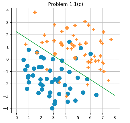
The data points given for problem 1.1 along with the decision boundary learned by logistic regression as executed by Newton’s method.
1.2 Poisson regression and the exponential family
1.2.1 Part (a)
Write the Poisson distribution as an exponential family:
\[p(y;\eta) = b(y)\exp\big(\eta^T T(y) - a(\eta)\big),\]
where
\[p(y;\lambda) = \frac{e^{-\lambda}\lambda^y}{y!}.\]
This can be done via
\[\begin{array}{rcl} \eta & = & \log(\lambda), \\ a(\eta) & = & e^\eta = \lambda, \\ b(y) & = & 1/y!, \text{ and} \\ T(y) & = & y. \end{array}\]
1.2.2 Part (b)
As is usual with generalized linear models, we’ll let \(\eta = {\theta}^Tx.\) The canonical response function is then given by
\[g(\eta) = E[y;\eta] = \lambda = e^\eta = e^{{\theta}^Tx}.\]
1.2.3 Part (c)
Based on the last part, I’ll define the hypothesis function \(h\) via \(h(x) = e^{{\theta}^Tx}.\)
For a single data point \((x, y),\) let \(\ell({\theta}) = \log(p(y|x)) =\) \(\log(\frac{1}{y!}) + (y{\theta}^T x-e^{{\theta}^Tx}).\) Then
\[\frac{\partial}{\partial{\theta}_j}\ell({\theta}) = yx_j - x_je^{{\theta}^Tx} = x_j(y-e^{{\theta}^Tx}).\]
So stochastic gradient ascent for a single point \((x, y)\) would use the update rule
\[{\theta}:= {\theta}+ \alpha x(y - h(x)).\]
1.2.4 Part (d)
In section 1.10 of my notes — the section on generalized linear models — I derived the update rule:
\[{\theta}:= {\theta}+ \alpha\big(T(y)-a'({\theta}^Tx)\big)x.\]
The missing piece is to proof that \(h(x) = E[y] = a'(\eta),\) which we’ll do next. We’ll work in the context of \(T(y)=y,\) as given by the problem statement. Notice that, for any \(\eta,\)
\[\int p(y)dy = \int b(y)\exp(\eta^Ty - a(\eta))dy = 1.\]
Since this identity is true for all values of \(\eta,\) we can take \(\frac{\partial}{\partial\eta}\) of it to arrive at the value 0:
\[\begin{array}{rcl} 0 & = & \frac{\partial}{\partial\eta}\int p(y)dy \\ & = & \int \frac{\partial}{\partial\eta} b(y)\exp(\eta^Ty - a(\eta))dy \\ & = & \int b(y)(y - a'(\eta))\exp(\eta^Ty - a(\eta)) dy \\ & = & \int y p(y)dy - a'(\eta)\int p(y)dy \\ & = & E[y] - a'(\eta). \end{array}\]
Thus we can conclude that \(E[y] = a'(\eta) = a'({\theta}^Tx),\) which completes the solution.
1.3 Gaussian discriminant analysis
1.3.1 Part (a)
This problem is to show that a two-class GDA solution effectively provides a model that takes the form of a logistic function, similar to logistic regression. This is something I already did in section 2.1 of my notes.
1.3.2 Parts (b) and (c)
These parts ask to derive the maximum likelihood estimates of \(\phi,\) \(\mu_0,\) \(\mu_1,\) and \(\Sigma\) for GDA. Part (b) is a special case of part (c), so I’ll just do part (c).
Some lemmas
It will be useful to know a couple vector- and matrix-oriented calculus facts which I’ll briefly derive here.
First I’ll show that, given column vectors \(a\) and \(b,\) and symmetric matrix \(C,\)
\[\nabla_b [ (a-b)^T C (a-b) ] = -2C(a-b).\qquad(1)\]
We can derive this by looking at the \(k^\text{th}\) coordinate of the gradient. Let \(x = (a-b)^T C (a-b).\) Then, using repeated index summation notation,
\[\begin{array}{crcl} & x & = & (a_i - b_i)c_{ij}(a_j-b_j) \\ \Rightarrow & [\nabla_b]_k x & = & -c_{kj}(a_j - b_j) - (a_i - b_i)c_{ik} \\ & & = & -2C(a-b). \\ \end{array}\]
Next I’ll show that
\[\frac{\partial}{\partial C}(a-b)^T C (a-b) = (a-b)(a-b)^T.\qquad(2)\]
This follows since
\[(a-b)^T C (a-b) = (a_i - b_i) c_{ij} (a_j - b_j),\]
so that
\[\frac{\partial}{\partial c_{ij}} (a-b)^T C (a-b) = (a_i - b_i)(a_j - b_j).\]
In other words, the \(ij^\text{th}\) entry of the matrix derivative is exactly the \(ij^\text{th}\) entry of the matrix \((a-b)(a-b)^T.\)
Finally, I’ll mention that, when a matrix \(A\) is invertibe,
\[\frac{d}{dA} |A| = |A|\,A^{-T}.\qquad(3)\]
This can be seen by considering that the \(ij^\text{th}\) entry of \(A^{-1}\) can be written as
\[(A^{-1})_{ij} = ((-1)^{i+j}M_{ji})/|A|,\qquad(4)\]
where \(M_{ij}\) denotes the determinant of the minor of \(A\) achieved by removing the \(i^\text{th}\) row and \(j^\text{th}\) column. Next, consider the expression for \(A\) as a sum of products \(\sigma(\pi)\prod a_{i\pi(i)}\) over all permutations \(\pi:[n]\to[n]\) where \(\sigma(\pi)\) is the sign of permutation \(\pi\) (reference). Based on that definition of a determinant, it can be derived that
\[\frac{\partial}{\partial a_{ij}}|A| = (-1)^{i+j}M_{ij}.\]
Combine this last result with (4) to arrive at (3).
The solution
We’re now ready to derive the equations for the GDA parameters based on maximum likelihood estimation.
The log likelihood function is
\[\ell = \sum_i \log(p(x|y)) + \log(p(y)).\]
\(\phi\)
In this section I’ll start to use the notation \([\textsf{Pred}(x)]\) for the indicator function of a boolean predicate \(\textsf{Pred}(x):\)
\[[\textsf{Pred}(x)] := \begin{cases} 1 & \text{if }\textsf{Pred}(x)\text{ is true, and} \\ 0 & \text{otherwise.} \\ \end{cases}\]
This is the notation that Knuth uses, and I prefer it to Ng’s notation \(1\{\textsf{Pred}(x)\}.\)
Treating \(p(y)\) as \(\phi^y(1-\phi)^{1-y},\) set \({\frac{\partial}{\partial \phi}}\) of \(\ell\) to 0; the result is
\[\sum_i{\frac{\partial}{\partial \phi}}\big(y\log\phi + (1-y)\log(1-\phi)\big) = \sum_i \frac{y}{\phi} - \frac{1-y}{1-\phi} = 0\]
\[\Rightarrow\quad \sum_i y(1-\phi) - (1-y)\phi = 0\]
\[\Rightarrow\quad m_1 - m_1\phi = m_0\phi,\]
where \(m_j = \sum_i [y{^{(i)}}= j],\) and I’m treating the possible \(y\) values as 0 or 1. Then
\[m_1 = \phi(m_0 + m_1) \;\Rightarrow\; \phi = \frac{m_1}{m},\]
using that \(m = m_0 + m_1.\)
\(\mu_j\)
\[{\frac{\partial}{\partial \mu_j}}\ell = {\frac{\partial}{\partial \mu_j}}\sum_{y=j}-\frac{1}{2}(x-\mu_j)^T{\Sigma^{-1}}(x-\mu_j)\]
We can use (1) to see that this is the same as
\[\sum_{y=j} {\Sigma^{-1}}(x-\mu_j).\]
Setting \({\frac{\partial}{\partial \mu_j}}\ell = 0,\) and noticing that \({\Sigma^{-1}}\) must be nonsingular as it’s an inverse, we get
\[\sum_{y=j} x = \sum_{y=j} \mu_j,\]
resulting in
\[ \sum_{y=j} x = m_j \mu_j \quad \Rightarrow \quad \mu_j = \frac{1}{m_j}\sum_{y=j}x .\]
\(\Sigma\)
To get an equation for \(\Sigma,\) we’ll actually maximize \(\ell\) with respect to its inverse \({\Sigma^{-1}}.\) This works because there is a bijection between all possible values of \({\Sigma^{-1}}\) and of \(\Sigma\) under the constraint that \(\Sigma\) is invertible, which is required for GDA to make sense. Thus the value of \({\Sigma^{-1}}\) which maximizes \(\ell\) uniquely identifies the value of \(\Sigma\) which maximizes \(\ell.\)
\[{\frac{\partial}{\partial {\Sigma^{-1}}}}\ell = \sum_i{\frac{\partial}{\partial {\Sigma^{-1}}}}\left(C + \frac{1}{2}\log |{\Sigma^{-1}}| - \frac{1}{2}(x-\mu_y)^T{\Sigma^{-1}}(x-\mu_y)\right).\]
Use (2) to see that this is the same as
\[\sum_i \frac{|{\Sigma^{-1}}|\Sigma^T}{|{\Sigma^{-1}}|} - \frac{1}{2}(x-\mu_y)(x-\mu_y)^T.\]
Set this value to 0 to arrive at
\[\sum_i \Sigma^T = \sum_i (x-\mu_y)(x-\mu_y)^T \quad\Rightarrow\quad \Sigma^T = \frac{1}{m}\sum_i (x-\mu_y)(x-\mu_y)^T.\]
Since the expression on the right must give a symmetric matrix, this same expression also gives the value for \(\Sigma\) itself.
1.4 Linear invariance of optimization algorithms
1.4.1 Part (a)
This problem is to show that Newton’s method is invariant to linear reparametrizations.
Specifically, suppose \(x^{(0)} = z^{(0)} = 0,\) that matrix \(A\) is invertible, and that \(g(z) = f(Az).\) Our goal is to show that if the sequence \(x^{(1)}, x^{(2)}, \ldots\) results from Newton’s method applied to \(f\), then the corresponding sequence \(z^{(1)}, z^{(2)}, \ldots\) resulting from Newton’s method applied to \(g\) obeys the equation \(x^{(i)} = Az^{(i)}\) for all \(i,\) so that the two versions of Newton’s method are in a sense doing the exact same work. We’ll think of \(f\) consistently as a function of \(x,\) and \(g\) as a function of \(z.\)
Start with
\[\big[\nabla_z g\big]_i = {\frac{\partial f}{\partial z_i}} = {\frac{\partial f}{\partial x_j}}{\frac{\partial x_j}{\partial z_i}} = {\frac{\partial f}{\partial x_j}}a_{ji},\]
from which it follows that
\[\nabla g = A^T\nabla f.\]
Next, introduce the variables \(H\) as the Hessian of \(f,\) and \(P\) as the Hessian of \(g.\) Then
\[ \begin{aligned} p_{ij} & = {\frac{\partial}{\partial z_i}}{\frac{\partial f}{\partial z_j}} = {\frac{\partial}{\partial z_i}}\left({\frac{\partial f}{\partial x_k}}a_{kj}\right) = \left({\frac{\partial}{\partial z_i}}{\frac{\partial f}{\partial x_k}}\right)a_{kj} \\ & = \left({\frac{\partial}{\partial x_\ell}}{\frac{\partial x_\ell}{\partial z_i}}{\frac{\partial f}{\partial x_k}}\right)a_{kj} = \left(a_{\ell i}\frac{\partial^2f}{\partial x_\ell\partial x_k}\right)a_{kj} = a_{\ell i}h_{\ell k}a_{kj}. \end{aligned} \]
We can summarize this as
\[P = A^T H A.\]
Newton’s method in this context can be expressed by the two equations
\[\begin{aligned} x^{(i+1)} & = x^{(i)} - H^{-1}(x^{(i)}) \nabla f(x^{(i)}), \text{ and} \\ z^{(i+1)} & = z^{(i)} - P^{-1}(z^{(i)}) \nabla g(z^{(i)}) \\ & = z^{(i)} - (A^THA)^{-1}(x^{(i)}) A^T\nabla f(x^{(i)}). \\ \end{aligned}\]
We’ll show by induction on \(i\) that \(x^{(i)} = Az^{(i)}\) for all \(i.\) The base case for \(i=0\) is true by definition. For the inductive step, assume that \(x^{(i)} = Az^{(i)},\) and use the above equations to see that
\[\begin{aligned} Az^{(i+1)} & = Az^{(i)} - AA^{-1}H(x^{(i)})A^{-T}A^T\nabla f(x^{(i)}) \\ & = x^{(i)} - H(x^{(i)}) \nabla f(x^{(i)}) \\ & = x^{(i+1)}, \end{aligned}\]
which completes this part of the problem.
1.4.2 Part (b)
Gradient descent is not invariant to linear reparametrizations. The update equation for \(f\) is
\[x^{(i+1)} = x^{(i)} - \alpha\nabla f,\]
and for \(g\) is
\[z^{(i+1)} = z^{(i)} - \alpha\nabla g = z^{(i)} - \alpha A^T\nabla f.\]
In order for \(Az^{(i+1)} = x^{(i+1)},\) we would need
\[A(z^{(i)} - \alpha A^T\nabla f) = Az^{(i)} - A\alpha\nabla f \quad\Leftrightarrow\quad AA^T\nabla f = A\nabla f,\]
but this is only guaranteed when \(A\) is unitary.
1.5 Regression for denoising quasar spectra
1.5.1 Part (a)
Let the \(i{^\text{th}}\) row of \(X\) be \(x{^{(i)}}.\) Then \((X{\theta})_i = \langle x{^{(i)}},{\theta}\rangle\) and \((X{\theta}- y)_i = \langle x{^{(i)}}, {\theta}\rangle - y{^{(i)}}.\)
Let the \(i{^\text{th}}\) diagonal element of \(W\) be \(\frac{w{^{(i)}}}{2}.\) Then \(((X{\theta}-y)^T W)_i = \frac{w{^{(i)}}}{2}(\langle x{^{(i)}},{\theta}\rangle-y{^{(i)}}\rangle)\) so that
\[J({\theta}) = (X{\theta}- y)^T W (X{\theta}- y) = \sum_i \frac{w{^{(i)}}}{2}(\langle x{^{(i)}},{\theta}\rangle - y{^{(i)}})^2.\]
This gives us a nice way to express \(J({\theta})\) in terms of matrices and vectors, as the problem requested.
This problem is to explicitly solve for \(\nabla_{\theta}J({\theta}) = 0\) for the function \(J({\theta})\) given in the last part.
I’ll begin by defining the general notation
\[\langle a, b \rangle_W := a^T W b.\]
This is similar to a standard inner product when both \(a\) and \(b\) are column vectors, but the notation still works when \(a\) or \(b\) are matrices of appropriate dimensions.
Let’s find some gradient formulas for \(\nabla_{\theta}\langle a, b\rangle_W\) in the case that \(a, b\) depend on \({\theta}\) but \(W\) doesn’t. It will be useful to keep in mind that
\[\langle a, b \rangle_W = a_i w_{ij} b_j.\]
Then
\[{\frac{\partial}{\partial {\theta}_k}}(a_i w_{ij} b_j) = a'_i w_{ij} b_j + a_i w_{ij} b'_j,\]
where \(x'\) denotes \({\frac{\partial x}{\partial {\theta}_k}}.\)
Define the matrix \(A'\) so that it has \(k{^\text{th}}\) column \({\frac{\partial}{\partial {\theta}_k}} a,\) and similarly for \(B'\) from \(b.\) Then
\[{\frac{\partial}{\partial {\theta}_k}}\langle a, b\rangle_W = \langle {\frac{\partial a}{\partial {\theta}_k}}, b \rangle_W + \langle a, {\frac{\partial b}{\partial {\theta}_k}} \rangle_W,\]
which we can summarize as
\[\nabla_{\theta}\langle a, b\rangle_W = \langle A',b \rangle_W + \langle a,B' \rangle_W^T.\]
In the special case that \(W\) is symmetric, we also have
\[\begin{aligned} \nabla_{\theta}\langle z, z \rangle_W & = \langle Z', z\rangle_W + \langle z, Z' \rangle_W^T \\ & = \langle Z', z\rangle_W + (z^T W Z')^T \\ & = \langle Z', z\rangle_W + Z'^T W z \\ & = 2 \langle Z', z\rangle_W, \\ \end{aligned}\]
which can be summarized as
\[\nabla_{\theta}\langle z, z \rangle_W = 2\langle Z', z\rangle_W.\]
To get back to the actual problem, notice that, by letting \(z = X{\theta}- y,\) we can write \(J = \langle z, z \rangle_W.\)
Then
\[\begin{aligned} \nabla J & = 2\langle Z', z\rangle_W \\ & = 2 Z'^T W z \\ & = 2 X^T W z \\ & = 2 X^T W (X {\theta}- y) = 0 \\ \Rightarrow \; X^T W X {\theta}& = X^T W y \\ \Rightarrow \; {\theta}& = (X^T W X)^{-1} X^T W y = (\langle X, X\rangle_W)^{-1} \langle X, y \rangle_W, \\ \end{aligned}\]
which is the closed-form expression the problem asked for.
In this problem, we suppose that
\[(y{^{(i)}}\mid x{^{(i)}}) \sim \mathcal N({\theta}^T x{^{(i)}}, \sigma{^{(i)}}).\]
Our goal is to show that maximizing the log likelihood in this scenario is the same as an application of weighted linear regression as seen in the previous two parts.
Begin by writing that
\[\begin{aligned} \ell({\theta}) & = \sum_i \log\left(c_i \exp\left( -\frac{(y{^{(i)}}- {\theta}^T x{^{(i)}})^2}{2(\sigma{^{(i)}})^2}\right)\right) \\ & = \sum_i \log(c_i) - \frac{(y{^{(i)}}- {\theta}^T x{^{(i)}})^2}{2(\sigma{^{(i)}})^2}, \end{aligned}\]
where \(c_i\) is a value independent of \({\theta},\) so that we may safely ignore it when taking \(\nabla_{\theta}.\)
From this point on I won’t write the \(i\) index on variables. I hope it’s clear from context. Then
\[\nabla_{\theta}\ell = \sum_i \frac{2(y - {\theta}^T x)x}{2\sigma^2},\]
so that \(\nabla\ell = 0\) when
\[\sum_i \frac{1}{\sigma^2}(y - {\theta}^T x)x = 0.\]
Let the \(k{^\text{th}}\) diagonal element of \(W\) be \(1/(\sigma^{(k)})^2,\) and define matrix \(X\) so that its \(i{^\text{th}}\) row is \(x{^{(i)}}.\) Also let \(\vec y\) denote the column vector with \(i{^\text{th}}\) coordinate \(y{^{(i)}}.\) Then
\[\sum_i \frac{1}{\sigma^2}(y - {\theta}^T x)x = X^T W (\vec y - X{\theta}).\]
This can be confirmed by seeing that the column vector \(m = W(\vec y - X{\theta})\) has \(i{^\text{th}}\) coordinate \(\frac{1}{(\sigma{^{(i)}})^2}(y{^{(i)}}- {\theta}^T x{^{(i)}}),\) and seeing the product \(X^T m\) as \(\sum_i x{^{(i)}}m_i.\)
But this last expression matches what we found in part ii of this problem, showing that solving this maximum likelihood estimate is effectively the same as solving a weighted linear regression problem.
1.5.2 Part (b)
i
I interpret this problem as applying linear regression to the first row of the given data file as a function of the wavelengths. This is the Python code I used:
#!/usr/bin/env python
"""Problem 1_5b_i.py

Graph the first row of data and a linear regression for
this data.
"""

import matplotlib.pyplot as plt
import numpy as np
import numpy.linalg as la


# Load the data.
all_data = np.loadtxt('quasar_train.csv', delimiter=',')
lambdas  = all_data[0, :]
data     = all_data[1:, :]
row1     = data[0, :]

# Run least squares.
A    = np.vstack((lambdas, np.ones(len(lambdas)))).T
m, c = la.lstsq(A, row1)[0]

# Plot the data and line.
plt.plot(lambdas, row1, 'o', label='spectra data',
    markersize=2)
plt.plot(lambdas, m * lambdas + c, 'r', label='fitted line')
plt.title('Problem 1.5(b)i')
plt.legend()
plt.show()
The code generated this image:
The first row of quasar spectra data plotted against wavelengths along with the line of best fit.
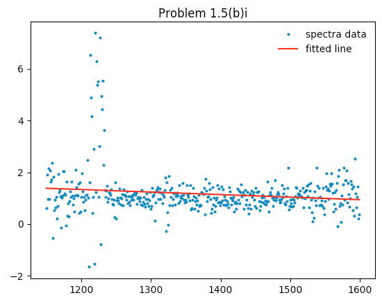
The line found had a slope of -0.000981122145459 with an intercept value of 2.5133990556. In other words, the spectra value \(v\) is approximated via the equation
\[v = 2.5134 - 9.8112\mathrm{e}{-4} \, \lambda,\]
where \(\lambda\) is the wavelength.
ii
Here is the code:
#!/usr/bin/env python
"""Problem 1_5b_ii.py
Graph the first row of data along with a locally weighted
linear regression.
"""
import matplotlib.pyplot as plt
import numpy as np
import numpy.linalg as la
# A function to solve locally weighted linear regression for
# given matrices X and W.
def lwlr_theta(X, W, y):
A = X.T.dot(W)
B = A.dot(X)
return la.inv(B).dot(A).dot(y)
def lwlr_at_pt(all_x, y, query_x):
X = np.vstack((np.ones(len(all_x)), all_x)).T
x = query_x
tau = 5
denom = 2.0 * tau ** 2
w = np.exp([-(x - xi) ** 2/denom for xi in all_x])
W = np.diag(w)
theta = lwlr_theta(X, W, y)
return theta[0] + theta[1] * query_x
def main():
# Load the data.
all_data = np.loadtxt('quasar_train.csv', delimiter=',')
lambdas = all_data[0, :]
data = all_data[1:, :]
row1 = data[0, :]
# Compute the LWLR curve at each lambda.
curve = [lwlr_at_pt(lambdas, row1, x) for x in lambdas]
# Plot the data and line.
plt.plot(lambdas, row1, 'o', label='spectra data',
markersize=2)
plt.plot(lambdas, curve, 'r', label='LWLR curve')
plt.title('Problem 1.5(b)ii')
plt.legend()
plt.show()
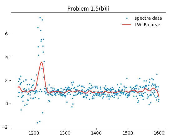
if __name__ == '__main__': main()Here is the graph generated:
The first row of quasar spectra data plotted against wavelengths along with the curve resulting from a locally weighted linear regression with \(\tau = 5.\)
iii
In this problem, we repeat part ii, except with the \(\tau\) values 1, 10, 100, and 1000.
The code is similar to the above. Here is the graph generated:
The first row of quasar spectra data plotted against wavelengths along with the curves resulting from locally weighted linear regressions with \(\tau = 1, 10, 100,\) and 1000.
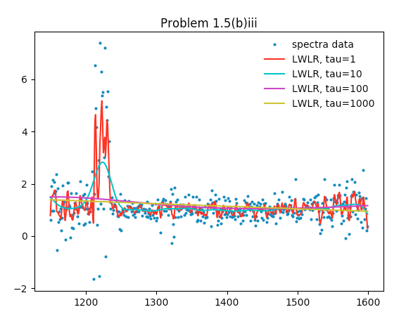
As \(\tau\) increases, the resulting LWLR curve becomes smoother. Smaller \(\tau\) values allow for more variation at a local level, thus fitting the data more closely, but also enabling wild variations due to noise.